Fluid Correlations and Other Calculations¶

A model is only as good as the correlations it is based on. A number of heat transfer and pressure drop correlations are needed for various components in the cycle. The table below summarizes the correlations used, and references are available for all the correlations.

Summary of correlations employed

Parameter	Reference
Single-phase pressure drop	Churchill [1]
Single-phase heat transfer	Gnielinski [2]
Two-phase pressure drop	Lockhart-Martinelli [3]
Two-phase evaporation heat transfer	Shah [4]
Two-phase condensation heat transfer	Shah [5]
Two-phase void fraction	Zivi [6]

Single-phase refrigerant pressure drop, heat transfer and charge¶

The Churchill correlation (based on a Darcy friction factor for which the laminar friction factor is $f=64/\mathrm{Re}_D$ ) is

(1) $A = \left(-2.457\log\left[\left(\frac{7}{\mathrm{Re}_D}\right)^{0.9} + 0.27 (\varepsilon/D) \right]\right)^{16}$

(2) $B = \left[\frac{37530.0}{\mathrm{Re}_D}\right]^{16}$

(3) $f = 8\left[\left(\frac{8}{\mathrm{Re}_D}\right)^{12} + \frac{1}{(A+B)^{1.5}} \right]^{1/12}$

with the Reynolds number defined by

(4) $\mathrm{Re}_D=\frac{\rho \bar U D}{\mu}=\frac{4\dot m}{\pi \mu D}$

With the known friction factor, the pressure gradient is given by

(5) $\frac{dp}{dz}=\frac{-fvG^2}{2D}$

with the mass flux defined by

(6) $G=\frac{\dot m}{(\pi D^2/4)}$

and assuming the gradient to be constant over the length L because averaged properties are used, the total pressure drop is

(7) $\Delta p=\frac{-fvG^2L}{2D}$

The Gnielinski correlation, good for smooth tubes and 0.5 < Pr < 2000 and 3000 < $\mathrm{Re}_D$ < $5x10^6$ , gives the single-phase heat transfer coefficient as

(8) $\alpha=\frac{k}{D} \mbox{ } \frac{(f/8)(\mathrm{Re}_D-1000)\Pr}{1+12.7(f/8)^{1/2}(\Pr^{2/3}-1)}$

The refrigerant charge for a single-phase volume is equal to

(9) $m=\rho V$

where the density $\rho$ is based on the average temperature and pressure.

In the case that given circuit of a heat exchanger is being analyzed, the value of $L$ is equal to the length of the circuit (or average length if there are multiple circuits). In addition, the mass flow rate $\dot m$ is therefore given as the mass flow rate per circuit.

Two-phase refrigerant pressure drop, heat transfer and charge¶

In the two-phase portion, the pressure drop components which are non-zero are the frictional pressure drop and the accelerational pressure drop. The gravitational pressure drop is also assumed to be negligible. In the case of evaporation, both frictional and acceleration result in a decrease in pressure. The Lockhart-Martinelli correlation is used to find the frictional pressure drop gradient, but it varies with quality. The total pressure drop is then found by integrating the pressure drop gradient over the range of qualities of interest.

Lockhart-Martinelli frictional pressure drop

The Lockhart-Martinelli two-phase pressure drop gradient is based on the following algorithm:

Find the Reynolds Number for each phase based on the actual flow rate of the individual phase

(10) $\mathrm{Re}_g=\frac{GxD}{\mu_g}$

(11) $\mathrm{Re}_f=\frac{G(1-x)D}{\mu_f}$
Friction factor for each phase

(12) $f_f=\left\lbrace \begin{array}{cc} \dfrac{16.0}{\mathrm{Re}_f} & \mathrm{Re}_f<1000 \\[1.0em] \dfrac{0.046}{\mathrm{Re}_f^{0.2}} & \mathrm{Re}_f>2000 \\[1.0em] w\dfrac{16.0}{\mathrm{Re}_f}+(1-w)\dfrac{0.046}{\mathrm{Re}_f^{0.2}} & 1000 < \mathrm{Re}_f < 2000 \end{array} \right.$

where $w=(\mathrm{Re}_f-1000)/(2000-1000)$ which results in a linear interpolation for the transitional Reynolds number region

(13) $f_g=\left\lbrace \begin{array}{cc} \dfrac{16.0}{\mathrm{Re}_g} & \mathrm{Re}_g<1000 \\[1.0em] \dfrac{0.046}{\mathrm{Re}_g^{0.2}} & \mathrm{Re}_g>2000 \\[1.0em] w\dfrac{16.0}{\mathrm{Re}_g}+(1-w)\dfrac{0.046}{\mathrm{Re}_g^{0.2}} & 1000 < \mathrm{Re}_g < 2000 \end{array} \right.$

where $w=(\mathrm{Re}_g-1000)/(2000-1000)$ which results in a linear interpolation for the transitional Reynolds number region
Frictional pressure drop based on actual flow rate of each phase

(14) $-\left(\dfrac{dp}{dz}\right)_f=\frac{2f_fG^2(1-x)^2v_f}{D}$

(15) $-\left(\dfrac{dp}{dz}\right)_g=\frac{2f_gG^2x^2v_g}{D}$
Lockhart-Martinelli parameter

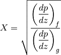
(16) $X=\sqrt{ \frac{\left(\dfrac{dp}{dz}\right)_f}{\left(\dfrac{dp}{dz}\right)_g} }$
Find the L-M Constant based on the flow Re of each phase (using 1500 as the transitional Re to ensure continuity)

(17) $C=\left\lbrace \begin{array}{cc} 20 & \mathrm{Re}_f>1500\mbox{ \& }\mathrm{Re}_g > 1500 \\ 12 & \mathrm{Re}_f<1500\mbox{ \& }\mathrm{Re}_g>1500 \\ 10 & \mathrm{Re}_f>1500\mbox{ \& }\mathrm{Re}_g<1500 \\ 5 & \mathrm{Re}_f< 1500\mbox{ \& }\mathrm{Re}_g<1500 \end{array} \right.$
Two-phase multipliers for each phase

Gas multiplier

(18) $\phi_g=1+CX+X^2$

Fluid multiplier

(19) $\phi_f=1+\frac{C}{X}+\frac{1}{X^2}$
Find gradient for a given value of $x$

(20) $-\left(\dfrac{dp}{dz}\right)_{f,2\phi}=\left\lbrace \begin{array}{lcr} -\left(\dfrac{dp}{dz}\right)_g\phi_g & & -\left(\dfrac{dp}{dz}\right)_g\phi_g> -\left(\dfrac{dp}{dz}\right)_f\phi_f \\ -\left(\dfrac{dp}{dz}\right)_f\phi_f & & -\left(\dfrac{dp}{dz}\right)_g\phi_g< -\left(\dfrac{dp}{dz}\right)_f\phi_f\end{array} \right.$
Average pressure drop gradient
Frictional pressure drop

Accelerational pressure drop

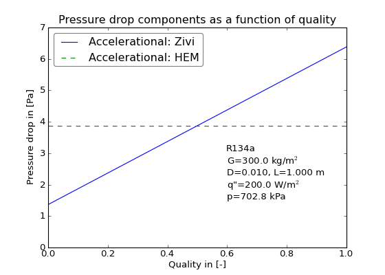
From the consideration of two-phase flow analysis, the accelerational presssure drop can be obtained. It is caused by the change in velocity of the vapor and liquid phases due to phase change, which in boiling creates vapor and accelerates the vapor, or in the case of condensation, reduces the vapor velocity, resulting in a pressure increase.

(21) $-\left( \frac{\partial p}{\partial z}\right)_A=G^2\frac{d}{dz}\left[\frac{x^2v_g}{\epsilon}+\frac{(1-x)^2v_f}{1-\epsilon}\right]$

where $\epsilon$ is the refrigerant vapor void fraction (typically the symbol $\alpha$ is used for void fraction, but here we are using that for heat transfer coefficient). Integrating over the length where the quality goes from $x_1$ to $x_2$ yields

(22) $\Delta p_A=\int_{0}^{L}\left[-\left( \frac{\partial p}{\partial z}\right)_A dz\right]$

(23) $\Delta p_A=L\left[\left(\frac{x_2^2v_g}{\epsilon_2}+\frac{(1-x_2)^2v_f}{1-\epsilon_2}\right) -\left(\frac{x_1^2v_g}{\epsilon_1}+\frac{(1-x_1)^2v_f}{1-\epsilon_1} \right) \right]$

where $\Delta p_A$ is positive if the pressure is dropping. If the quality in the term

(24) $\left(\frac{x^2v_g}{\epsilon}+\frac{(1-x)^2v_f}{1-\epsilon} \right)$

is 0 or 1, one part is zero and the other is an indeterminate form of 0/0. One evaluation of L’Hopital’s rule can be used to show that if the quality is zero, the term in Equation (24) is equal to $v_f$ , or if the quality is 1, this term is equal to $v_g$ .

(Source code)

(png, hires.png, pdf)

(png, hires.png, pdf)

(png, hires.png, pdf)

Shah Condensation

The liquid-only heat transfer coefficient is given by: (25) $\alpha_L = 0.023 \left(\frac{GD}{\mu_f} \right)^{0.8} \mathrm{Pr}_f^{0.4} \frac{k_f}{D}$

And the overall heat transfer coefficient for a given quality $x$ is given by

(26) $\alpha_{2\phi}(x)=\alpha_L \left((1 - x)^{0.8} + \frac{3.8 x^{0.76} (1 - x)^{0.04}}{(p^*)^{0.38}} \right)$

where $p^*=p_{sat}/p_{crit}$ . The average condensation heat transfer coefficient between a quality of $x_1$ and $x_2$ is given by

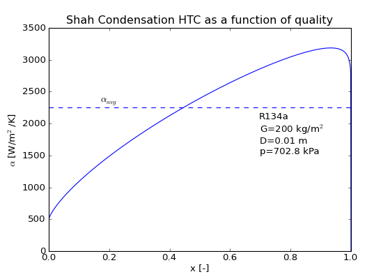
(27) $\overline{\alpha_{2\phi}}=\dfrac{\int_{x_1}^{x_2} [\alpha_{2\phi}(x)dx]}{x_2-x_1}$

where the integral is evaluated numerically using adaptive quadrature. A sample plot of the heat transfer coefficient as a function of quality is shown here:

(Source code, png, hires.png, pdf)

Shah Evaporation

This correlation is used to model the heat transfer coefficient for boiling fluid in a tube.

The non-dimensional groups of interest are the convection number

(28) $\mathrm{Co} = \left(\frac{1}{x} - 1\right)^{0.8} \sqrt{\frac{\rho_g}{\rho_f}}$

the Froude number

(29) $\mathrm{Fr}_l = \frac{G^2}{\rho_f^2gD}$

and the boiling number

(30) $\mathrm{Bo} = \frac{q"}{Gh_{fg}}$

The pure-liquid heat transfer coefficient is given by

(31) $\alpha_l = 0.023 \left(\frac{G (1 - x) D}{ \mu_f}\right)^{0.8} \mathrm{Pr}_f^{0.4} \frac{k_f}{D}$

If Bo > 0.0011 then F = 14.7, otherwise F = 15.43

If $\mathrm{Fr}_l \geq 0.04$ then N = Co, else $N = 0.38\mathrm{Fr}_l^{-0.3}Co$

(32) $\psi_{cb} = \frac{1.8}{N^{0.8}}$

If N is between 0.1 and 1.0 inclusive

(33) $\psi_{bs} = F \sqrt{\mathrm{Bo}} \exp(2.74 N^{-0.1}) \psi = \max(\psi_{bs}, \psi_{cb})$

If N<0.1

(34) $\psi_{bs} = F \sqrt{\mathrm{Bo}} \exp(2.47 N^{-0.15}) \psi = \max(\psi_{bs}, \psi_{cb})$

If N is very small in magnitude, $\exp(2.47 N^{-0.15})$ blows up to infinity, so to correct, at high vapor quality, the value for the heat transfer coefficient between quality of 0.999 and 1.0 is linearly interpolated to give better behavior at very high vapor quality (which yields very small values of N). The pure vapor (x=1) heat transfer coefficient is given by

(35) $\alpha_g = 0.023 \left(\frac{G D}{ \mu_g}\right)^{0.8} \mathrm{Pr}_g^{0.4} \frac{k_g}{D}$

If N > 1.0 and Bo > 0.00003

(36) $\psi_{nb} = 230 \sqrt{\mathrm{Bo}} \psi = \max(\psi_{nb},\psi_{cb})$

If N > 1.0 and Bo < 0.00003

(37) $\psi_{nb} = 1.0 + 46.0 \sqrt{\mathrm{Bo}} \psi = \max(\psi_{nb},\psi_{cb})$

(38) $\alpha_{2\phi}(x)=\psi \alpha_l$

The average evaporation heat transfer coefficient between a quality of $x_1$ and $x_2$ is given by

(39) $\overline{\alpha_{2\phi}}=\frac{\int_{x_1}^{x_2} [\alpha_{2\phi}(x)dx]}{x_2-x_1}$

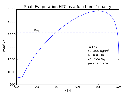
where the integral is evaluated numerically. A sample plot of the heat transfer coefficient as a function of quality is shown here:

(Source code, png, hires.png, pdf)

Refrigerant Charge

Using the Zivi slip flow model, the slip ratio is equal to

(40) $S=\left(\frac{v_g}{v_f}\right)^{1/3}$

which yields the void fraction for a given quality of

(41) $\epsilon=\frac{1}{1+\frac{\rho_g}{\rho_f}S\left(\frac{1-x}{x}\right)}$

and the average void fraction between qualities of $x_1$ and $x_2$ can be given by

(42) $\overline{\epsilon}=-{{C_{\epsilon}\,\left(\log \left({{\left({x_2}-1\right)\,C_{\epsilon}-{x_2} }\over{\left({x_1}-1\right)\,C_{\epsilon}-{x_1}}}\right)+ {x_2}-{x_1}\right)-{x_2}+{x_1}}\over{\left( {x_2}-{x_1}\right)\,C_{\epsilon}^2+\left(2\,{x_1}-2\, {x_2}\right)\,C_{\epsilon}+{x_2}-{ x_1}}}$

where the term $C_{\epsilon}$ is given by

(43) $C_{\epsilon}=\frac{\rho_g}{\rho_f}S$

which yields the average density in the two-phase portion of

(44) $\overline{\rho}=\rho_g\overline{\epsilon}+\rho_f(1-\overline{\epsilon})$

Thus the total mass contained in the two-phase section is equal to

(45) $m=\bar{\rho}V$

References

Nomenclature

Variable	Description
$A$	Coefficient for friction factor equation [-]
$B$	Coefficient for friction factor equation [-]
$\mathrm{Bo}$	Boiling number [-]
$C$	Coefficient in L-M equation [-]
$C_{\epsilon}$	Coefficient in L-M equation [-]
$\mathrm{Co}$	Convection number [-]
$D$	Diameter [m]
$f$	Friction factor [-]
$f_f$	Friction factor [-]
$f_g$	Friction factor [-]
$F$	Coefficient in Shah Evaporation [-]
$\mathrm{Fr}_l$	Froude number [-]
$g$	Gravitational constant [m/s²]
$G$	Mass flux [kg/m²/s]
$k$	Thermal conductivity [W/m/K]
$k_f$	Saturated liquid thermal conductivity [W/m/K]
$L$	Length [m]
$\dot m$	Mass flow rate [kg/s]
$m$	Mass [kg]
$N$	Coefficient in Shah Evaporation [-]
$p$	Pressure [kPa]
$p^*$	Reduced pressure [-]
$q"$	Heat flux [W/m²]
$\mathrm{Pr}$	Prandtl Number
$\mathrm{Pr}_f$	Prandtl number of saturated liquid [-]
$\mathrm{Re}_D$	Reynolds number based on diameter [-]
$\mathrm{Re}_f$	Reynolds number of saturated liquid [-]
$\mathrm{Re}_g$	Reynolds number of saturated vapor [-]
$S$	Slip ratio [-]
$\bar U$	Average velocity [m/s]
$V$	Volume [m³]
$v$	Specific volume [m³/kg]
$v_f$	Specific volume of saturated liquid [m³/kg]
$v_g$	Specific volume of saturated vapor [m³/kg]
$w$	L-M weighting parameter in transitional region [-]
$x$	Quality [-]
$X$	Lockhart-Martinelli parameter [-]
$z$	Position [m]
$\alpha$	Heat transfer coefficient [W/m²/K]
$\alpha_L$	Liquid heat transfer coefficient [W/m²/K]
$\alpha_{2\phi}$	Two-phase heat transfer coefficient [W/m²/K]
$\varepsilon$	Surface roughness [m]
$\epsilon$	Void fraction [-]
$\phi_g$	Frictional multiplier [-]
$\phi_f$	Frictional multiplier [-]
$\mu$	Viscosity [Pa-s]
$\mu_f$	Viscosity of saturated liquid [Pa-s]
$\mu_g$	Viscosity of saturated vapor [Pa-s]
$\psi_{bs}$	Coefficient [-]
$\psi_{nb}$	Nucleate boiling coefficient [-]
$\psi_{cb}$	Convective boiling coefficient [-]
$\rho$	Density [kg/m³]
$\rho_f$	Density of saturated liquid [kg/m³]
$\rho_g$	Density of saturated vapor [kg/m³]

[1]	Churchill, S.W., Friction-factor equation spans all fluid-flow regimes, Chemical Engineering v. 84, n. 24 91-92

[2]	Gnielinski, V., 1976, New Equation for Heat and Mass Transfer in Turbulent Pipe and Channel Flow, Int. Chemical Engineering v. 16, 359-368.

[3]	Lockhart, R.W., Martinelli, R.C., 1949, Proposed Correlation of Data for Isothermal Two-Phase Two-Component Flow in Pipes. Chemical Engineering Progress. v. 45, 39-48

[4]	Shah, M., 1976. A New Correlation for Heat Transfer During Boiling Flow Through Pipes. ASHRAE Transactions 82, 66-86.

[5]	Shah, M., 1979. A general correlation for heat transfer during film condensation inside pipes. International Journal of Heat and Mass Transfer 22, 547-556.

[6]	Zivi, S., 1964. Estimation of Steady-State Void-Fraction by Means of the Principle of Minimum Entropy Production. Journal of Heat Transfer 86, 247-252.

Fluid Correlations and Other Calculations¶

Single-phase refrigerant pressure drop, heat transfer and charge¶

Two-phase refrigerant pressure drop, heat transfer and charge¶

Table Of Contents

Previous topic

Next topic

This Page

Navigation

Fluid Correlations and Other Calculations¶

Single-phase refrigerant pressure drop, heat transfer and charge¶

Two-phase refrigerant pressure drop, heat transfer and charge¶

Table Of Contents

Previous topic

Next topic

This Page

Quick search

Navigation