Cycle Solver¶

In the cycle solver, the goal is to use all the physical component models together in order to obtain the performance of the combined cycle. The process is slightly different for each of the 4 standard configurations of ACHP, but there are many common themes among the configurations. ACHP has been designed to investigate direct expansion (DX) systems as well as systems employing a secondary working loop, in both cooling and heating modes.

A number of simplifying assumptions are employed at the cycle level:

Pressure drops in each component are calculated, but not used directly(see Pressure-Drop Correction for explanation)
There is no charge inventory in the compressor shell
The evaporator outlet refrigerant superheat is imposed (implies an expansion device with perfect superheat control)
No pressure drops except for in the components considered

Direct Expansion Cooling Mode¶

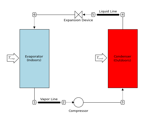
The most common and straightforward system is the direct expansion cooling mode system. The schematic of this cycle is shown in this figure:

(Source code, png, hires.png, pdf)

In addition to the geometry of each component, required inputs are the superheat at the outlet of the evaporator $\Delta T_{sh,evap}$ , and either the total refrigerant charge $m_r$ or the refrigerant subcooling at the outlet of the condenser $\Delta T_{sc,cond}$ .

The primary independent variables in the cycle solver are the saturation temperatures of the refrigerant at evaporation and condensation, given by $T_{evap}$ and $T_{cond}$ respectively. For pure refrigerants the saturation temperature for a given pressure is the same for saturated liquid and saturated vapor. For pseudo-pure fluids and blends, the refrigerant dew temperature is used which corresponds to saturated vapor.

Before the full cycle-solver is run, the preconditioner in section Cycle Solver Preconditioner is used to get a good guess for the temperatures $T_{evap}$ and $T_{cond}$ using extremely simple cycle models.

Once the preconditioner has been run, preliminary values for $T_{evap}$ and $T_{cond}$ are known, and the first iteration of the cycle model may begin. Execution of the cycle model follows in the same direction as the refrigerant flow. The pressure drops through low-pressure and high-pressure parts of the system are assumed to be zero initially.

The cycle analysis begins with the vapor line which returns refrigerant vapor from the evaporator that is typically in the air duct back to the condensing unit outdoors. In the first iteration of the cycle solver, the mass flow rate of refrigerant in the vapor line is not known, but the compressor map is used to provide a reasonable guess value for the mass flow rate of refrigerant. The Line Set model is used to calculate the process from point 1 to point 2. The model is run with known flow rates and an inlet temperature of $T_{evap}+\Delta T_{sh}$ in order to calculate the state at the inlet to the compressor.

The compressor compresses refrigerant from state point 2 to state point 3. The Compressor model is used which is based on an empirical correlation with superheat correction and it yields the outlet state 3 as well as the compressor mass flow rate, compressor electrical power, etc.. The compressor model requires the temperatures $T_{evap}$ and $T_{cond}$ as well as the compressor inlet superheat.

The condenser takes the superheated refrigerant at state point 3 and condenses it to a subcooled refrigerant at state point 4. The Condenser model is used to calculate the process, and this condenser model is based on a moving-boundary model. The condenser model requires $T_{cond}$ as an input, among others.

After the condenser, the subcooled refrigerant passes through the liquid-line that takes refrigerant from the condenser to the indoor coil that is inside the ductwork in the home. The Line Set model is used to model the flow that passes from state point 4 to state point 5.

The expansion device then expands the refrigerant from the high-pressure side of the system to the low-pressure side of the system. In the current iteration of ACHP, no expansion device is included. Thus the expansion device is just a constant-enthalpy throttling device that takes refrigerant from the high-side pressure at state point 5 to the low-side pressure at state point 6.

At the outlet of the expansion device, the refrigerant passes into the evaporator at some two-phase quality. The Evaporator model is used to model the performance of the evaporator. In the evaporator, refrigerant is heated by the air-stream (which cools the air stream) from state point 6 back to state point 1’, which should be superheated (note: not necessarily so at intermediate iterations of cycle model) close to state point 1. If the values of the cycle independent variables $T_{evap}$ and $T_{cond}$ have been well selected, the state points 1 and 1’ will be coincident.

Once the cycle model has been run around the loop from state point 1 to state point 1’, the residuals can be calculated. The residuals are terms that when the cycle model has converged should all be equal to zero.

One of the residuals that is always active is an energy balance over the cycle. You left from state point 1, and you should hopefully arrive back there if energy is conserved in the cycle. Thus, the first residual is given by

(1) $\vec \Delta_1=\dot m_r(h_1-h_{1'})$

where $h_1$ and $h_{1'}$ are the enthalpies of the refrigerant at state points 1 and 1’ respectively.

Since there are two independent variables, there must be a second constraint, which in this case is a charge-level constraint. Either the charge is constrained directly with an imposed charge level, or indirectly with an imposed refrigerant subcooling. Thus the second residual can be given by

(2) $\vec \Delta_2=\left \lbrace \begin{array}{cc} m_r-m_{r,target} & (\mbox{Charge imposed}) \\ \Delta T_{sc}-\Delta T_{sc,target} & (\mbox{Subcooling imposed})\end{array} \right .$

and a numerical solver is used to drive the residual vector $\vec \Delta$ to sufficiently close to zero by altering $T_{evap}$ and $T_{cond}$ (see Multi-dimensional solver).

Pressure-Drop Correction¶

After the cycle model has iterated to convergence, the pressure drops are then considered. In reality, the pressure drop in each component results in a lower pressure at the inlet of the next component in the refrigerant loop. In terms of modeling, coupling pressure drop and the component models causes great numerical difficulties. The compromise that is employed instead is to run all the component models without pressure drop, but calculate the high-side pressure drop as the pressure drop of the condenser and liquid-line:

(3) $\Delta p_{high}=\Delta p_{cond}+\Delta p_{liquid-line}$

and similarly, the low-side pressure drop is defined by

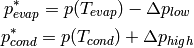
(4) $\Delta p_{low}=\Delta p_{evap}+\Delta p_{vapor-line}$

These pressure drops are then employed to shift the saturation temperatures used in the compressor map in order to yield less refrigerant mass flow rate, and a higher compressor power.

The new effective compressor suction and discharge pressures are

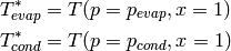
(5) $p_{evap}^*=p(T_{evap})-\Delta p_{low} p_{cond}^*=p(T_{cond})+\Delta p_{high}$

and the new, effective compressor dew temperatures are

(6) $T_{evap}^*=T(p=p_{evap},x=1) T_{cond}^*=T(p=p_{cond},x=1)$

This calculated pressure drop is used until the model reaches convergence again, at which point the pressure drop tems are updated, and the model is run again. This process continues until the imposed low- and high-side pressure drops are equal to the pressure drop terms calculated from the converged cycle model.

Cycle Performance Parameters¶

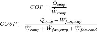
The common metrics of system efficiency are

(7) $COP=\frac{\dot Q_{evap}}{\dot W_{comp}} COSP=\frac{\dot Q_{evap}-\dot W_{fan,evap}}{\dot W_{comp}+\dot W_{fan,evap}+\dot W_{fan,cond}}$

from Cycle import DXCycleClass

#Instantiate the cycle class
Cycle=DXCycleClass()

#--------------------------------------
#       Cycle parameters
#--------------------------------------
Cycle.Verbosity = 0 #the idea here is to have different levels of debug output
Cycle.ImposedVariable = 'Subcooling'                                                           
Cycle.DT_sc_target = 7.0
Cycle.Mode='AC' 
Cycle.Ref='R410A'

#--------------------------------------
#       Compressor parameters
#--------------------------------------

#A 3 ton cooling capacity compressor map 
M=[217.3163128,5.094492028,-0.593170311,4.38E-02,-2.14E-02,
    1.04E-02,7.90E-05,-5.73E-05,1.79E-04,-8.08E-05]
P=[-561.3615705,-15.62601841,46.92506685,-0.217949552,
    0.435062616,-0.442400826,2.25E-04,2.37E-03,-3.32E-03,2.50E-03]

params={
    'M':M,
    'P':P,
    'Ref':Cycle.Ref,  #Refrigerant
    'fp':0.0, #Fraction of electrical power lost as heat to ambient
    'Vdot_ratio': 1.0, #Displacement Scale factor                  
    'Verbosity': 0, # How verbose should the debugging be [0-10]
  }
Cycle.Compressor.Update(**params)                                          

#--------------------------------------
#      Condenser parameters 
#--------------------------------------
Cycle.Condenser.Fins.Tubes.NTubes_per_bank=24  #number of tubes per bank=row
Cycle.Condenser.Fins.Tubes.Nbank=1             #number of banks/rows
Cycle.Condenser.Fins.Tubes.Ncircuits=3
Cycle.Condenser.Fins.Tubes.Ltube=2.252
Cycle.Condenser.Fins.Tubes.OD=0.00913
Cycle.Condenser.Fins.Tubes.ID=0.00849
Cycle.Condenser.Fins.Tubes.Pl=0.0191  #distance between center of tubes in flow direction                                                
Cycle.Condenser.Fins.Tubes.Pt=0.0254  #distance between center of tubes orthogonal to flow direction

Cycle.Condenser.Fins.Fins.FPI=25      #Number of fins per inch
Cycle.Condenser.Fins.Fins.Pd=0.001    #2* amplitude of wavy fin
Cycle.Condenser.Fins.Fins.xf=0.001    #1/2 period of fin
Cycle.Condenser.Fins.Fins.t=0.00011   #Thickness of fin material
Cycle.Condenser.Fins.Fins.k_fin=237   #Thermal conductivity of fin material

Cycle.Condenser.Fins.Air.Vdot_ha=1.7934 #rated volumetric flowrate
Cycle.Condenser.Fins.Air.Tmean=308.15   
Cycle.Condenser.Fins.Air.Tdb=308.15     #Dry Bulb Temperature
Cycle.Condenser.Fins.Air.p=101.325      #Air pressure
Cycle.Condenser.Fins.Air.RH=0.51        #Relative Humidity
Cycle.Condenser.Fins.Air.RHmean=0.51
Cycle.Condenser.Fins.Air.FanPower=260

Cycle.Condenser.Ref=Cycle.Ref
Cycle.Condenser.Verbosity=0
    
#--------------------------------------
#     Evaporator Parameters
#--------------------------------------
Cycle.Evaporator.Fins.Tubes.NTubes_per_bank=32
Cycle.Evaporator.Fins.Tubes.Nbank=3
Cycle.Evaporator.Fins.Tubes.Ltube=0.452
Cycle.Evaporator.Fins.Tubes.OD=0.00913
Cycle.Evaporator.Fins.Tubes.ID=0.00849
Cycle.Evaporator.Fins.Tubes.Pl=0.0191
Cycle.Evaporator.Fins.Tubes.Pt=0.0254
Cycle.Evaporator.Fins.Tubes.Ncircuits=5

Cycle.Evaporator.Fins.Fins.FPI=14.5
Cycle.Evaporator.Fins.Fins.Pd=0.001
Cycle.Evaporator.Fins.Fins.xf=0.001
Cycle.Evaporator.Fins.Fins.t=0.00011
Cycle.Evaporator.Fins.Fins.k_fin=237

Cycle.Evaporator.Fins.Air.Vdot_ha=0.56319
Cycle.Evaporator.Fins.Air.Tmean=297.039
Cycle.Evaporator.Fins.Air.Tdb=297.039
Cycle.Evaporator.Fins.Air.p=101.325
Cycle.Evaporator.Fins.Air.RH=0.5
Cycle.Evaporator.Fins.Air.RHmean=0.5
Cycle.Evaporator.Fins.Air.FanPower=438
       
Cycle.Evaporator.Ref=Cycle.Ref
Cycle.Evaporator.Verbosity=0
Cycle.Evaporator.DT_sh=5

# ----------------------------------
#       Line Set Parameters
# ----------------------------------
params={
    'L':7.6,
    'k_tube':0.19,
    't_insul':0.02,
    'k_insul':0.036,
    'T_air':297,
    'Ref': Cycle.Ref,
    'h_air':0.0000000001,
}

Cycle.LineSetSupply.Update(**params)
Cycle.LineSetReturn.Update(**params)
Cycle.LineSetSupply.OD=0.009525
Cycle.LineSetSupply.ID=0.007986
Cycle.LineSetReturn.OD=0.01905
Cycle.LineSetReturn.ID=0.017526

#Now solve
from time import time
t1=time()
Cycle.PreconditionedSolve()
print 'Took '+str(time()-t1)+' seconds to run Cycle model'
print 'Cycle coefficient of system performance is '+str(Cycle.COSP)
print 'Cycle refrigerant charge is '+str(Cycle.Charge)+' kg'

which should yield the output, when run, of

Took 0.90700006485 seconds to run Cycle model
Cycle coefficient of system performance is 3.07586682038
Cycle refrigerant charge is 2.01022253223 kg

Direct Expansion Heating Mode¶

The heat pump configuration of the system is as shown here:

(Source code, png, hires.png, pdf)

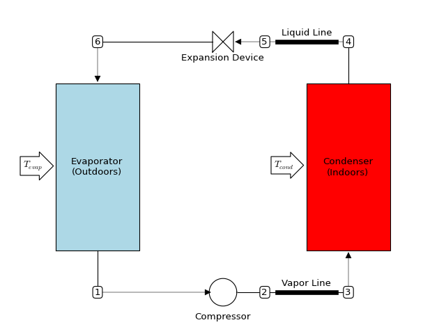
Physically, reversing valves are used to switch the mode of the system and the directions of the flows. What was the condenser of the air conditioning system becomes the evaporator of the heat pump and vice versa, and the line sets are configured in a slightly different way. Other than that, the analysis of the heat pump is directly analogous to that of the Direct Expansion Cooling Mode system.

A Preconditioner is used to get approximate values for $T_{evap}$ and $T_{cond}$ , and using these values (which are iteratively modified using numerical methods), the solution for the cycle performance is found.

As with the cooling mode, the cycle analysis follows the refrigerant flow path around the loop.

Beginning at the outlet of the evaporator, state point 1 is known because $T_{evap}$ and $\Delta T_{sh}$ are known. Thus the compressor model is used directly to calculate the electrical power, refrigerant mass flow rate and state point 2.

The Line Set model is then applied to the flow from the outlet of the compressor at state point 2 to the inlet of the condenser at state point 3.

The Condenser model is used to model the condensing process from state point 3 to a subcooled state at state point 4.

The Line Set model is used to model the flow of subcooled refrigerant at state point 4 back to the expansion device at state point 5.

As in cooling mode, the expansion device is assumed to be an ideal expansion device, which means that the working process is a constant-enthalpy expansion from state point 5 to state point 6.

The Evaporator model is then used to calculate the evaporation process of refrigerant from state point 6 to state point 1’.

As in cooling mode, the residual vector is given by

(8) $\vec \Delta=[\vec \Delta_1, \vec \Delta_2]$

with

(9) $\vec \Delta_1=\dot m_r(h_1-h_{1'}) \vec \Delta_2=\left \lbrace \begin{array}{cc} m_r-m_{r,target} & (\mbox{Charge imposed}) \\ \Delta T_{sc}-\Delta T_{sc,target} & (\mbox{Subcooling imposed})\end{array} \right .$

The set of $T_{evap}$ and $T_{cond}$ which solve the residual equations are obtained by a multi-dimensional solver (see Multi-dimensional solver).

Cycle Performance Parameters¶

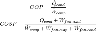
The common metrics of system efficiency are

(10) $COP=\frac{\dot Q_{cond}}{\dot W_{comp}} COSP=\frac{\dot Q_{cond}+\dot W_{fan,cond}}{\dot W_{comp}+\dot W_{fan,evap}+\dot W_{fan,cond}}$

from Cycle import DXCycleClass,F2K

#Instantiate the class
Cycle=DXCycleClass()

#--------------------------------------
#       Cycle parameters
#--------------------------------------
Cycle.Verbosity = 0 #the idea here is to have different levels of debug output
Cycle.ImposedVariable = 'Subcooling' #or it could be 'Charge'
Cycle.DT_sc_target = 7.0
#Cycle.Charge_target = 3.3 #uncomment for use with imposed charge
Cycle.Mode='HP' 
Cycle.Ref='R410A'

#--------------------------------------
#       Compressor parameters
#--------------------------------------

#A few 3 ton cooling capacity compressor maps 
M=[217.3163128,5.094492028,-0.593170311,4.38E-02,
    -2.14E-02,1.04E-02,7.90E-05,-5.73E-05,1.79E-04,-8.08E-05]
P=[-561.3615705,-15.62601841,46.92506685,-0.217949552,
    0.435062616,-0.442400826,2.25E-04,2.37E-03,-3.32E-03,2.50E-03]

params={
'M':M,
'P':P,
'Ref':Cycle.Ref,                                                              #refrigerant
'fp':0.0, #Fraction of electrical power lost as heat to ambient            #shell heat loss
'Vdot_ratio': 1.0, #Displacement Scale factor                               #up- or downsize compressor (1=original)
'Verbosity': 0, # How verbose should the debugging statements be [0 to 10]                        
}
Cycle.Compressor.Update(**params)                                          

#--------------------------------------
#      Condenser parameters 
#--------------------------------------
Cycle.Condenser.Fins.Tubes.NTubes_per_bank=32
Cycle.Condenser.Fins.Tubes.Nbank=3
Cycle.Condenser.Fins.Tubes.Ncircuits=6
Cycle.Condenser.Fins.Tubes.Ltube=0.452
Cycle.Condenser.Fins.Tubes.OD=0.009525
Cycle.Condenser.Fins.Tubes.ID=0.0089154
Cycle.Condenser.Fins.Tubes.Pl=0.0254
Cycle.Condenser.Fins.Tubes.Pt=0.0219964

Cycle.Condenser.Fins.Fins.FPI=14.5
Cycle.Condenser.Fins.Fins.Pd=0.001
Cycle.Condenser.Fins.Fins.xf=0.001
Cycle.Condenser.Fins.Fins.t=0.00011
Cycle.Condenser.Fins.Fins.k_fin=237

Cycle.Condenser.Fins.Air.Vdot_ha=0.5663
Cycle.Condenser.Fins.Air.Tmean=F2K(70)
Cycle.Condenser.Fins.Air.Tdb=F2K(70)
Cycle.Condenser.Fins.Air.p=101.325
Cycle.Condenser.Fins.Air.RH=0.51
Cycle.Condenser.Fins.Air.RHmean=0.51
Cycle.Condenser.Fins.Air.FanPower=438

Cycle.Condenser.Ref=Cycle.Ref
Cycle.Condenser.Verbosity=0

#--------------------------------------
#           Evaporator parameters
#--------------------------------------
Cycle.Evaporator.Fins.Tubes.NTubes_per_bank=41  #number of tubes per bank=row
Cycle.Evaporator.Fins.Tubes.Nbank=1             #number of banks/rows
Cycle.Evaporator.Fins.Tubes.Ncircuits=5
Cycle.Evaporator.Fins.Tubes.Ltube=2.286
Cycle.Evaporator.Fins.Tubes.OD=0.007
Cycle.Evaporator.Fins.Tubes.ID=0.0063904
Cycle.Evaporator.Fins.Tubes.Pl=0.0191  #distance between center of tubes in flow direction                                                
Cycle.Evaporator.Fins.Tubes.Pt=0.0222  #distance between center of tubes orthogonal to flow direction

Cycle.Evaporator.Fins.Fins.FPI=25      #Number of fins per inch
Cycle.Evaporator.Fins.Fins.Pd=0.001    #2* amplitude of wavy fin
Cycle.Evaporator.Fins.Fins.xf=0.001    #1/2 period of fin
Cycle.Evaporator.Fins.Fins.t=0.00011   #Thickness of fin material
Cycle.Evaporator.Fins.Fins.k_fin=237   #Thermal conductivity of fin material

Cycle.Evaporator.Fins.Air.Vdot_ha=1.7934 #rated volumetric flowrate
Cycle.Evaporator.Fins.Air.Tmean=F2K(47)   
Cycle.Evaporator.Fins.Air.Tdb=F2K(47)     #Dry Bulb Temperature
Cycle.Evaporator.Fins.Air.p=101.325      #Air pressure
Cycle.Evaporator.Fins.Air.RH=0.51        #Relative Humidity
Cycle.Evaporator.Fins.Air.RHmean=0.51
Cycle.Evaporator.Fins.Air.FanPower=160

Cycle.Evaporator.Ref=Cycle.Ref
Cycle.Evaporator.Verbosity=0
Cycle.Evaporator.DT_sh=5

# ----------------------------------
#       Line Set parameters
# ----------------------------------
params={
'L':7.6,
'k_tube':0.19,
't_insul':0.02,
'k_insul':0.036,
'T_air':297,
'Ref': Cycle.Ref,
'h_air':6,
}

Cycle.LineSetSupply.Update(**params)
Cycle.LineSetReturn.Update(**params)
Cycle.LineSetSupply.OD=0.01905 
Cycle.LineSetSupply.ID=0.017526
Cycle.LineSetReturn.OD=0.009525
Cycle.LineSetReturn.ID=0.007986

#Now solve
from time import time
t1=time()
Cycle.PreconditionedSolve()

#Outputs
print 'Took '+str(time()-t1)+' seconds to run Cycle model'
print 'Cycle coefficient of system performance is '+str(Cycle.COSP)
print 'Cycle refrigerant charge is '+str(Cycle.Charge)+' kg'

which should yield the output, when run, of

Took 1.26699995995 seconds to run Cycle model
Cycle coefficient of system performance is 3.44174832875
Cycle refrigerant charge is 1.6918624607 kg

class Cycle.DXCycleClass[source]¶

Calculate(DT_evap, DT_cond)[source]¶

Inputs are differences in temperature [K] between HX air inlet temperature and the dew temperature for the heat exchanger.

Required Inputs:

DT_evap:: Difference in temperature [K] between evaporator air inlet temperature and refrigerant dew temperature
DT_cond:: Difference in temperature [K] between condenser air inlet temperature and refrigeant dew temperature

OutputList()[source]¶

Return a list of parameters for this component for further output

It is a list of tuples, and each tuple is formed of items:: [0] Description of value [1] Units of value [2] The value itself

PreconditionedSolve()[source]¶

Solver that will precondition by trying a range of DeltaT until the model can solve, then will kick into 2-D Newton Raphson solve

The two input variables for the system solver are the differences in temperature between the inlet air temperature of the heat exchanger and the dew temperature of the refrigerant. This is important for refrigerant blends with temperature glide during constant-pressure evaporation or condensation. Good examples of common working fluid with glide would be R404A or R410A.

Secondary Loop Cooling Mode¶

(Source code, png, hires.png, pdf)

For secondary loops in cooling mode, there is an internal heat exchanger which physically separates the secondary loop and the refrigerant loop.

In this case, there are now three inputs, and three residuals (to be defined later). The three inputs are $T_{g,i,cc}$ , $T_{evap}$ and $T_{cond}$ .

The two loops can be solved separately, where for the secondary loop, the inlet temperature to the cooling coil is known, and the secondary working fluid’s properties are independent of pressure.

To begin, the Cooling Coil model is employed to calculate the heat transfer rate in the cooling coil, which gives the process from state point 5 to state point 6.

The Line Set model is used to determine the heat transfer and pressure drop in the line going from state point 6 to state point 7.

The pump model is run to determine how much electrical power is consumed in the pump, which gives the state point 8, the glycol inlet to the internal heat exchanger.

The refrigerant loop is then solved. The refrigerant superheat at the outlet of the IHX is imposed as an input for the cycle. Thus state point 1 is known, and the Compressor model is used to calculate state point 2, the compressor mass flow rate, electrical power, etc..

The Condenser model is then solved using the state point 2 as the inlet, and yielding the (hopefully) subcooled refrigerant outlet state point 3.

Finally, the isenthalpic throttling process is used to determine the state point 4 at the refrigerant inlet to the IHX.

Lastly, the Plate-Heat-Exchangers model is run, using the inputs at state points 8 and 4, and yielding the refrigerant outlet state of state point 1’.

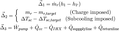
The residuals are given by an energy balance between state points 1 and 1’, an energy balance on the secondary loop, and either matching the mass or the subcooling on the refrigerant side. As in the DX system analysis, the residual vector is given by

(11) $\vec \Delta=[\vec \Delta_1, \vec \Delta_2, \vec \Delta_3]$

with

(12) $\vec \Delta_1=\dot m_r(h_1-h_{1'}) \vec \Delta_2=\left \lbrace \begin{array}{cc} m_r-m_{r,target} & (\mbox{Charge imposed}) \\ \Delta T_{sc}-\Delta T_{sc,target} & (\mbox{Subcooling imposed})\end{array} \right . \vec \Delta_3=\dot W_{pump}+\dot Q_{cc}-\dot Q_{IHX}+\dot Q_{\mathrm{suppply line}}+\dot Q_{\mathrm{return line}}$

The set of $T_{g,i,cc}$ , $T_{evap}$ and $T_{cond}$ which solve the residual equations are obtained by a multi-dimensional solver (see Multi-dimensional solver).

from Cycle import SecondaryCycleClass

#Instantiate the class
Cycle=SecondaryCycleClass()

#--------------------------------------
#       Cycle parameters
#--------------------------------------
Cycle.Verbosity = 0 #the idea here is to have different levels of debug output
Cycle.ImposedVariable = 'Subcooling' #or this could be 'Charge' for imposed charge
Cycle.DT_sc_target = 7.0
#Cycle.Charge_target = 2.4  #Needed if charge is imposed, not otherwise
Cycle.Ref='R410A'
Cycle.SecLoopFluid = 'EG-20%'
Cycle.IHXType = 'PHE'# or could be 'Coaxial'
Cycle.Mode='AC'

#--------------------------------------
#--------------------------------------
#       Compressor parameters
#--------------------------------------
#--------------------------------------

#A 3 ton cooling capacity compressor map
if Cycle.Ref=='R410A':
    M=[217.3163128,5.094492028,-0.593170311,4.38E-02,-2.14E-02,1.04E-02,
    7.90E-05,-5.73E-05,1.79E-04,-8.08E-05]
    P=[-561.3615705,-15.62601841,46.92506685,-0.217949552,0.435062616,
    -0.442400826,2.25E-04,2.37E-03,-3.32E-03,2.50E-03]

params={
    'M':M,
    'P':P,
    'Ref':Cycle.Ref,    #refrigerant
    'fp':0.15, #Fraction of electrical power lost as heat to ambient            
    'Vdot_ratio': 1.0, #Displacement Scale factor to up- or downsize compressor (1=original)
    'Verbosity': 0, # How verbose should the debugging statements be [0 to 10]
  }
Cycle.Compressor.Update(**params)

#--------------------------------------
#      Condenser parameters 
#--------------------------------------
Cycle.Condenser.Fins.Tubes.NTubes_per_bank=24  #number of tubes per bank=row
Cycle.Condenser.Fins.Tubes.Nbank=1             #number of banks/rows
Cycle.Condenser.Fins.Tubes.Ncircuits=3
Cycle.Condenser.Fins.Tubes.Ltube=2.252
Cycle.Condenser.Fins.Tubes.OD=0.00913
Cycle.Condenser.Fins.Tubes.ID=0.00849
Cycle.Condenser.Fins.Tubes.Pl=0.0191  #distance between center of tubes in flow direction                                                
Cycle.Condenser.Fins.Tubes.Pt=0.0254  #distance between center of tubes orthogonal to flow direction

Cycle.Condenser.Fins.Fins.FPI=25      #Number of fins per inch
Cycle.Condenser.Fins.Fins.Pd=0.001    #2* amplitude of wavy fin
Cycle.Condenser.Fins.Fins.xf=0.001    #1/2 period of fin
Cycle.Condenser.Fins.Fins.t=0.00011   #Thickness of fin material
Cycle.Condenser.Fins.Fins.k_fin=237   #Thermal conductivity of fin material

Cycle.Condenser.Fins.Air.Vdot_ha=1.7934 #rated volumetric flowrate
Cycle.Condenser.Fins.Air.Tmean=308.15   
Cycle.Condenser.Fins.Air.Tdb=308.15     #Dry Bulb Temperature
Cycle.Condenser.Fins.Air.p=101.325      #Air pressure
Cycle.Condenser.Fins.Air.RH=0.51        #Relative Humidity
Cycle.Condenser.Fins.Air.RHmean=0.51
Cycle.Condenser.Fins.Air.FanPower=260

Cycle.Condenser.Ref=Cycle.Ref
Cycle.Condenser.Verbosity=0
    
#--------------------------------------
#      Cooling Coil parameters
#--------------------------------------
Cycle.CoolingCoil.Fins.Tubes.NTubes_per_bank=32
Cycle.CoolingCoil.Fins.Tubes.Nbank=3
Cycle.CoolingCoil.Fins.Tubes.Ncircuits=5
Cycle.CoolingCoil.Fins.Tubes.Ltube=0.452
Cycle.CoolingCoil.Fins.Tubes.OD=0.00913
Cycle.CoolingCoil.Fins.Tubes.ID=0.00849
Cycle.CoolingCoil.Fins.Tubes.Pl=0.0191
Cycle.CoolingCoil.Fins.Tubes.Pt=0.0254

Cycle.CoolingCoil.Fins.Fins.FPI=14.5
Cycle.CoolingCoil.Fins.Fins.Pd=0.001
Cycle.CoolingCoil.Fins.Fins.xf=0.001
Cycle.CoolingCoil.Fins.Fins.t=0.00011
Cycle.CoolingCoil.Fins.Fins.k_fin=237

Cycle.CoolingCoil.Fins.Air.Vdot_ha=0.56319
Cycle.CoolingCoil.Fins.Air.Tmean=297.039
Cycle.CoolingCoil.Fins.Air.Tdb=297.039
Cycle.CoolingCoil.Fins.Air.p=101.325
Cycle.CoolingCoil.Fins.Air.RH=0.5
Cycle.CoolingCoil.Fins.Air.RHmean=0.5
Cycle.CoolingCoil.Fins.Air.FanPower=438
       
params={
    'Ref_g': Cycle.SecLoopFluid,
    'pin_g': 200,
    'Verbosity':0,
    'mdot_g':0.38
}
Cycle.CoolingCoil.Update(**params)

params={
    'ID_i':0.0278,
    'OD_i':0.03415,
    'ID_o':0.045,
    'L':50,
    'pin_g':300,
    'Ref_r':Cycle.Ref,
    'Ref_g':Cycle.SecLoopFluid,
    'Verbosity':0
    }
Cycle.CoaxialIHX.Update(**params)

params={
    'pin_h':300,
    'Ref_h':Cycle.SecLoopFluid,
    'Ref_c':Cycle.Ref,
    
    #Geometric parameters
    'Bp' : 0.117,
    'Lp' : 0.300, #Center-to-center distance between ports
    'Nplates' : 46,
    'PlateAmplitude' : 0.001, #[m]
    'PlateThickness' : 0.0003, #[m]
    'PlateConductivity' : 15.0, #[W/m-K]
    'PlateWavelength' : 0.00628, #[m]
    'InclinationAngle' : 3.14159/3,#[rad]
    'MoreChannels' : 'Hot', #Which stream gets the extra channel, 'Hot' or 'Cold'
    'Verbosity':0,
    'DT_sh':5
}
Cycle.PHEIHX.Update(**params)

params={
    'eta':0.5,  #Pump+motor efficiency
    'mdot_g':0.38, #Flow Rate kg/s
    'pin_g':300,
    'Ref_g':Cycle.SecLoopFluid,
    'Verbosity':0,
    }
Cycle.Pump.Update(**params)

params={
    'L':5,
    'k_tube':0.19,
    't_insul':0.02,
    'k_insul':0.036,
    'T_air':297,
    'Ref': Cycle.SecLoopFluid,
    'pin': 300,
    'h_air':0.0000000001,
}

Cycle.LineSetSupply.Update(**params)
Cycle.LineSetReturn.Update(**params)
Cycle.LineSetSupply.OD=0.009525
Cycle.LineSetSupply.ID=0.007986
Cycle.LineSetReturn.OD=0.01905
Cycle.LineSetReturn.ID=0.017526

#Now solve
from time import time
t1=time()
Cycle.PreconditionedSolve()

#Outputs
print 'Took '+str(time()-t1)+' seconds to run Cycle model'
print 'Cycle coefficient of system performance is '+str(Cycle.COSP)
print 'Cycle refrigerant charge is '+str(Cycle.Charge)+' kg'

which should yield the output, when run, of

Took 0.670000076294 seconds to run Cycle model
Cycle coefficient of system performance is 2.74883933092
Cycle refrigerant charge is 1.45798524528 kg

Secondary Loop Heating Mode¶

This section is left intentionally empty

Cycle Solver Class Documentation¶

class Cycle.SecondaryCycleClass[source]¶

Calculate(DT_evap, DT_cond, Tin_CC)[source]¶

Inputs are differences in temperature [K] between HX air inlet temperature and the dew temperature for the heat exchanger.

Required Inputs:

DT_evap:: Difference in temperature [K] between cooling coil air inlet temperature and refrigerant dew temperature
DT_cond:: Difference in temperature [K] between condenser air inlet temperature and refrigerant dew temperature
Tin_CC:: Inlet “glycol” temperature to line set feeding cooling coil

OutputList()[source]¶

Return a list of parameters for this component for further output

It is a list of tuples, and each tuple is formed of items:: [0] Description of value [1] Units of value [2] The value itself

PreconditionedSolve()[source]¶

Cycle Solver¶

Direct Expansion Cooling Mode¶

Pressure-Drop Correction¶

Cycle Performance Parameters¶

Direct Expansion Heating Mode¶

Cycle Performance Parameters¶

Secondary Loop Cooling Mode¶

Secondary Loop Heating Mode¶

Cycle Solver Class Documentation¶

Table Of Contents

Previous topic

Next topic

This Page

Navigation

Cycle Solver¶

Direct Expansion Cooling Mode¶

Pressure-Drop Correction¶

Cycle Performance Parameters¶

Direct Expansion Heating Mode¶

Cycle Performance Parameters¶

Secondary Loop Cooling Mode¶

Secondary Loop Heating Mode¶

Cycle Solver Class Documentation¶

Table Of Contents

Previous topic

Next topic

This Page

Quick search

Navigation